Predicting & Visualizing Hourly Electricity Demand in the US with MindsDB and Tableau

Credit: How To Visualize MindsDB Predictions with Tableau by EphraimX

Introduction

MindsDB is an open-source machine-learning tool that brings automated machine learning to your database. MindsDB offers predictive capabilities in your database. Tableau lets you visualize your data easily and intuitively. In this tutorial, we will be using MindsDB to predict the hourly electricity demand in the United States and visualize results in Tableau. To complete this tutorial, you are required to have a working MindsDB connection, either locally or via cloud.mindsdb.com. You can use this guide to connect to the MindsDB cloud.

Data Setup

Connecting the data as a file

Follow the steps below to upload a file to MindsDB Cloud.

• Log in to your MindsDB Cloud account to open the MindsDB Editor.
• Navigate to Add data the section by clicking the Add data button located in the top right corner.

• Choose the Files tab.

• Choose the Import File option.
• Upload a file (Demand for United States Lower 48 (region) hourly - UCT- time.csv), name a table used to store the file data (here it is US_Electricity_Demand), and click the Save and Continue button.

Once you are done uploading, you can query the data directly with;

SELECT * FROM files.US_Electricity_Demand LIMIT 10;

The output would be:

Understanding the Dataset

Whether you wonder to know how the electricity demand is evolving in the US during the year or you would like to know how the electricity mix has evolved through time, that’s the dataset for you!

Energy is always something we have taken for granted, but in recent years with all the bottlenecks and geopolitical problems that have followed one another, it has become an increasingly central theme.

You can get the dataset on Kaggle here and use the Demand for United States Lower 48 (region) hourly - UCT- time.csv.

Creating the Predictor

To being, let’s create a predictor that uses the date to predict the hourly energy consumption. You can learn more about creating a predictor by checking here. You can predict a timestamp series model using the following syntax

CREATE PREDICTOR mindsdb.[predictor_name]
FROM [integration_name]
    (SELECT [sequential_column], [partition_column], [other_column], [target_column]
     FROM [table_name])
PREDICT [target_column]

ORDER BY [sequential_column]
GROUP BY [partition_column]

WINDOW [int]
HORIZON [int];

• CREATE PREDICTOR: Creates a predictor with the name predictor_name in the mindsdb table.
• FROM files: Points to the table containing the data.
• PREDICT Close: Dictates the column to predict.
• ORDER BY: Shows the column to arrange the data during training.
• GROUP BY: It is optional. The column by which rows that make a partition are grouped. For example, if you want to forecast the inventory for all items in the store, you can partition the data by product_id, so each distinct product_idhas its own time series.
• WINDOW: Decides how many rows to "look back" into when creating a prediction.
• HORIZON: Specifies the number of future predictions. The default is 1.

Let’s proceed to make predictions on our dataset:

CREATE PREDICTOR mindsdb.hourly_electricity_demand
FROM files (SELECT * FROM US_Electricity_Demand)
PREDICT megawatthours
ORDER by date
-- the target column to be predicted stores one row per quarter
WINDOW 100      -- using data from the 100 rows to make forecasts 
HORIZON 20;    -- making forecasts for the next years

On execution we get:

Query successfully completed

Status of a Predictor

A predictor may take a couple of minutes for the training to complete. You can monitor the status of the predictor by using this SQL command:

SELECT status
FROM mindsdb.predictors
WHERE name='hourly_electricity_demand';

If we run it right immediately after creating a predictor, we get this output:

+------------+
| status     |
+------------+
| generating |
+------------+

After a while you will get:

+------------+
| status     |
+------------+
| training   |
+------------+

And finally, this should be your output:

+------------+
| status     |
+------------+
| complete   |
+------------+

Making Predictions

Now that we have our Prediction Model, we can simply execute some simple SQL query statements to predict the target value based on the feature parameters:

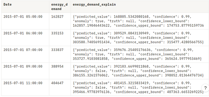
SELECT date, megawatthours AS `energy_demand` ,energy_demand_explain
FROM mindsdb.hourly_electricity_demand
JOIN files.US_Electricity_Demand
LIMIT 5;

Expected output would be:

You can also check the predictor’s accuracy with the query below to see how it performs.

SELECT accuracy
FROM mindsdb.predictors
WHERE name = 'hourly_electricity_demand'

Ouput:

+------------+
| accuracy   |
+------------+
| 0.992      |
+------------+

The accuracy score ranges from 0 to 1, and from the result, the model will be accurate 90% of the time.

Connecting MindsDB to Tableau

Tableau lets you visualize your data easily and intuitively. In this tutorial will use Tableau to create visualizations of our predictions.

How to Connect

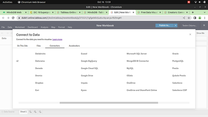
• First, create a new workbook in Tableau and open the Connectors tab in the Connect to Data window.
• Click on MySQL

• Input “cloud.mindsdb.com” for Server, “3306” for Port, “mindsdb” for Database “your mindsdb cloud email” for Username, “your mindsdb cloud password” for Password, and Sign in.

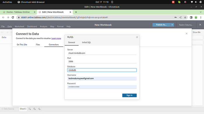
Now you are connected and your page should look like this:

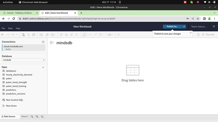
Visualizing our Data

Before you can visualize predictions in Tableau, you must first choose a data source. And because the predictions in this article are generated using a SQL statement, you will need to create a custom SQL query in Tableau to generate the data source. To do this:

• First, select the New Custom SQLon the left side of the window and use the query below to generate the energy demand for each hour. You can preview the results or directly load the data into Tableau.

SELECT date, megawatthours AS `energy_demand`
FROM mindsdb.hourly_electricity_demand
JOIN files.US_Electricity_Demand

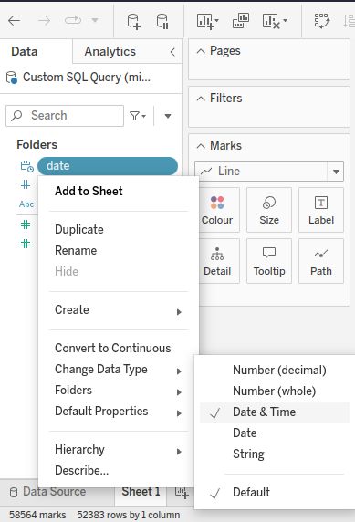
• Move to the Sheet tab and right-click on the energy_demand and date to convert their data types to Number(whole) and Date and Time, respectively. Additionally, when right-clicking on the enerygy_demand and data, choose the option to convert it to a continuous measure.

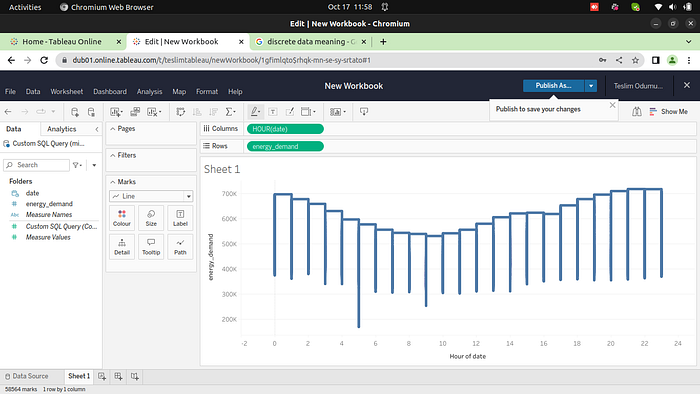
• Drag the energy_demand measure to the row shelf and the date dimension to the column shelf

Conclusion

In this tutorial, we created our own Mindsdb Cloud, uploaded a dataset to the interface, create a predictor model and visualize it on Tableau.

Have fun while trying it out yourself!

• Star the MindsDB repository on GitHub.
• Sign up for a free MindsDB account
• Engage with the MindsDB community on Slack or GitHub to ask questions and share your ideas and thoughts.

Give a like or a comment if this tutorial was helpful